How to estimate storage growth with writes, replication, and retention
A practical guide to calculating storage from writes per second, average data size, replication factor, and retention time before volume becomes cost or bottlenecks in production.
storage
capacity planning
systems design
software architecture
scalability
databases
Ednaldo Luiz
Level: Intermediate
Level:
Published:
Last updated:
Recommended
Resources related to storage estimation and capacity planning.
Software Engineer focused on architecture and performance. I work with Java/Spring Boot, well-structured SQL, scalable services on AWS, and GenAI solutions with RAG (LangChain + vector databases). I value readable code and well-justified decisions.
You know when everything seems fine, until the bill arrives? Storage goes over budget, and nobody can explain where the last few terabytes came from.
Storage almost never looks like a problem in the beginning. But data has a habit: it accumulates — one log here, one event there, every single day.
What looks small per second can become dozens of gigabytes per day and several terabytes per year — especially when replication, retention, backups, and history enter the picture.
That is why estimating storage is not about making a perfect calculation. It is about seeing the order of magnitude before growth becomes cost, a bottleneck, or a production incident. The goal is to be prepared for growth, not to guess the exact number.
TL;DR
Estimating storage means building the calculation in layers, with each layer multiplying the previous one:
writes/s × average size = data generated per second
It does not need to be exact. It only needs to be good enough to reveal the order of magnitude and prevent growth, retention, and replication from becoming surprises in production.
Before thinking about databases, disks, , backups, or any specific technology, we need to answer a more basic question: how fast is the system producing data?
This first calculation depends on two pieces of information:
how many writes happen per second;
the average size of each write.
With those two values, we can calculate the system's data generation rate. We are not considering retention time, replication, indexes, backups, or internal database structures yet. At this point, we only want to understand how much new data is produced every second.
It is not the final estimate, but it is the starting point for every other calculation.
The first step is to find out how many operations actually generate persisted data every second.
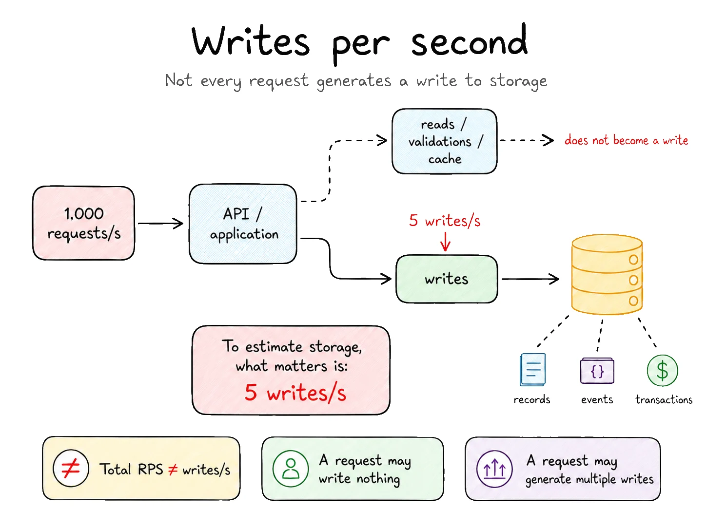
There is an important difference between and writes per second: they are not the same thing.
A system may receive 1,000 requests per second, but a large part of them may be reads, validations, cache lookups, or operations that do not persist anything.
The opposite can also happen. A single request can generate multiple writes. Creating an order, for example, may write the order, its items, an audit event, a message to a queue, and a structured log.
To estimate storage, what matters is the number of operations that actually produce data that will be stored.
In practice, writes/s comes from a measurement using real system metrics or from a traffic estimate — active users (DAU) → requests → writes. But the traffic calculation is a separate exercise; here, we start directly from writes.
Suppose the system performs:
This means five new records, events, transactions, or documents are produced every second.
Next, we need to understand how much each write weighs.
This value can vary a lot depending on the type of data. A simple event may have only a few kilobytes. A transaction with more information may be larger. A structured log can grow quickly. A file, image, or document changes the scale of the calculation completely.
For a first estimate, we use an average size.
For example:
This number does not need to be perfect at the beginning. The goal is to find an order of magnitude.
It is also important to remember: here we are talking about logical data, meaning the approximate size of the information being written. Indexes, replicas, backups, , journals, snapshots, or any internal storage overhead are not included yet.
Even so, this estimate already helps a lot. It is better to work with an approximate number than to ignore growth or assume storage is not a problem until it becomes one.
With those two pieces of information, the base calculation looks like this:
Write rate
Average size
Data generation
writes per second
×
average size per write
=
data generated per second
Write rate
writes per second
×
Using our example:
Write rate
Average size
Data generation
5 writes/s
×
50 KB
=
250 KB/s
Write rate
5 writes/s
×
Average size
250 KB looks small. And by itself, it really is.
But we are talking about just one second and an apparently small load: five writes of 50 KB. When that same pace continues throughout the entire day, every day, the volume stops looking so harmless.
The storage problem usually does not come from a single write. It comes from accumulation.
Now that we have the data generation rate, we can bring time into the calculation.
Now that we know how much data the system produces per second, we need to understand what happens when that pace continues for hours, days, months, or years.
This is when apparently small numbers start growing quickly — and also when calculations become full of zeros, conversions, and different units.
Approximation and scientific notation help with exactly that: they simplify the calculation without hiding the real scale of the problem. Instead of looking for absolute precision from the first step, we can quickly reach a useful estimate and understand where the volume is heading.
In an initial capacity estimate, the goal is to discover the order of magnitude of the problem. We want to know whether the system will produce megabytes, gigabytes, terabytes, or petabytes. At this stage, getting a perfectly exact number is usually less important than completing the calculation and understanding its scale.
A day has exactly 86,400 seconds. To simplify a quick estimate, we can round that value:
In our example, the system produces 250 KB of data per second. If it keeps that pace for approximately 100,000 seconds, we can estimate the daily volume.
Approximate calculation
1
Estimating volume in KB
250 KB/s × 100,000 seconds = 25,000,000 KB
We multiply the data generation rate by the approximate number of seconds in a day.
2
Converting KB to GB
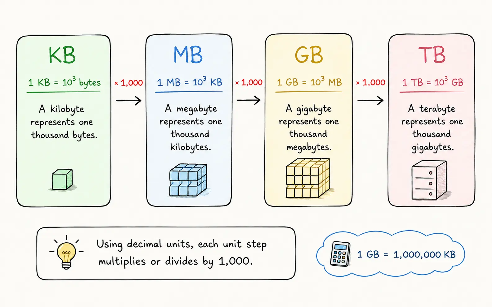
25,000,000 KB ÷ 1,000,000 = 25 GB per day
We divide by 1,000,000 because, in decimal units, 1 GB equals 1,000 MB and 1 MB equals 1,000 KB. Therefore, 1 GB = 1,000,000 KB.
3
Interpreting the result
25 GB per day
The value is still approximate, but the scale is already clear: we are talking about dozens of gigabytes produced per day.
This estimate uses 100,000 seconds as an approximation for one day.
The important part here is not memorizing powers of 10, but seeing the scale of the problem. If you prefer to calculate with the full numbers — 250 × 100,000 — instead of 10⁵, that is fine: you reach the same place. What matters is not letting the notation block the reasoning.
In the quick calculation, we used 10⁵ seconds to represent a day. That shortcut gave us an estimate of 25 GB per day.
Now let's redo the same calculation using the real number of seconds in a day: 86,400.
Calculation with real seconds
1
Volume in KB
250 KB/s × 86,400 seconds = 21,600,000 KB
Here we use the real number of seconds in a day, without rounding it to 100,000.
2
Conversion to GB
21,600,000 KB ÷ 1,000,000 = 21.6 GB per day
We divide by 1,000,000 because, in decimal units, 1 GB equals 1,000,000 KB.
With the shortcut, we got 25 GB/day. With the real number of seconds, we got 21.6 GB/day.
The general conclusion is still similar: in both cases, the system is producing dozens of gigabytes per day. But that does not mean the difference can always be ignored.
Quick estimate
More precise calculation
Difference
25 GB/day
Using 10⁵ seconds as an approximation for one day.
21.6 GB/day
Using the real 86,400 seconds in a day.
3.4 GB/day
Small in one day, but relevant when accumulated.
Quick estimate
25 GB/day
Using 10⁵ seconds as an approximation for one day.
More precise calculation
This is the important caution: a small difference per day can become a large difference when accumulated. Those 3.4 GB/day become roughly 100 GB/month and more than 1 TB/year — and that is still without considering replication, backups, snapshots, indexes, additional logs, or longer retention.
Even so, using 86,400 seconds does not make the estimate perfect. It only removes one rounding step from the calculation.
In practice, several other variables are still changing.
The system may receive less traffic on weekends, have peaks during business hours, grow during campaigns, specific dates, or month-end processing. The average data size can also change as new fields, logs, events, and integrations enter the system.
So approximation does not mean carelessness. It is a first reading of the scale of the problem, not a capacity guarantee.
When the decision involves cloud budget, disk limits, backups, , provisioning, or a customer commitment, we need to refine the calculation with real metrics, traffic patterns, and scenarios closer to production.
The rule of thumb is simple:
Use approximations to understand scale, and more precise values to make commitments.
We will keep using 25 GB/day as the base to follow the calculation. When the decision involves budget or provisioning, replace it with a real measurement or a more precise calculation, such as 21.6 GB/day.
Knowing how much data the system produces per day is still not enough.
To keep the calculation simple, we will continue with the quick estimate of 25 GB per day. The next question is: how long does this volume need to remain stored?
That answer changes the estimate completely. Keeping data for 7 days is one thing. Keeping it for 1 year is another. Keeping it for 5 years changes the size of the problem entirely.
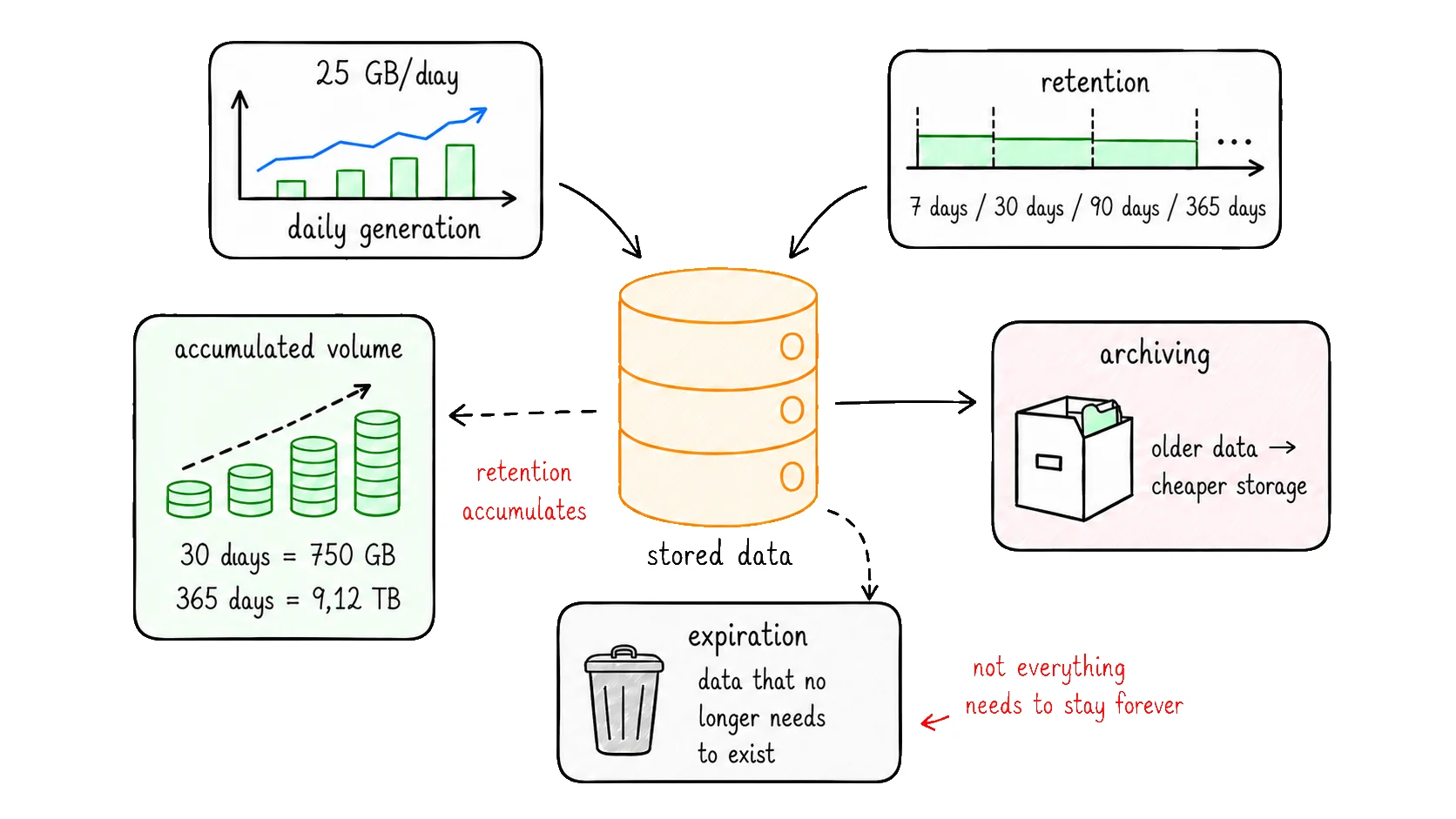
Retention time is exactly that: the period during which a piece of data must remain available before it is removed, archived, or moved to another type of storage.
Retention is a policy that defines how long each type of data will be kept.
Not all data needs to be stored for the same amount of time. Technical logs may have short retention. Audit events may need to stay for months or years. User-uploaded files may need to exist while the account is active. Financial, tax, or contractual data may depend on business rules, support, compliance, or legal obligations.
Some common examples:
Data type
Typical retention
Why this period matters
Technical logs
7, 15, 30, or 90 days
Investigation, debugging, and observability — they do not always need to stay forever.
Audit events
months or years
Needed to trace important actions in the system.
User files
as long as it makes sense for the product
Depends on the plan, contract, usage, or account lifecycle.
Tax or contractual data
years
Depends on legal, accounting, or regulatory obligations.
The important point is: retention is not just a technical choice. It depends on the product, the business, the operation, and in some cases, legal requirements.
So before estimating storage, we need to understand which data will be kept and for how long.
So far, we have reached a daily generation of approximately 25 GB per day.
To discover the accumulated volume, we multiply that value by the retention time.
Daily volume
Retention
Logical storage
25 GB/day
×
30 days
=
750 GB
Daily volume
25 GB/day
×
Retention
Now the number starts changing scale.
The 250 KB/s rate, which looked small at the beginning, became 25 GB per day. With only 30 days of retention, this already represents 750 GB of accumulated logical data.
If retention is longer, the impact grows with it.
Retention
Accumulated volume
What it represents
7 days
175 GB
Short retention, common for temporary data.
30 days
750 GB
One month of stored data.
90 days
2.25 TB
Three months already move the calculation into terabytes.
365 days
9.12 TB
One year completely changes the order of magnitude.
The same write rate can generate very different estimates depending on the retention time.
This is one of the most important parts of the estimate: storage does not grow only because the system receives more data per second. It grows because that data remains accumulated.
A common mistake is assuming that everything that was written must stay forever in the primary storage.
In practice, mature systems usually separate data by age, importance, and access frequency.
Recent data usually needs to remain more accessible, because it is queried more often by the product, support, reporting, or operations. Older data can be archived, compressed, aggregated, or moved to cheaper storage. Data that no longer needs to exist can be removed.
A simple data lifecycle strategy can be split into three layers:
Recent data
Older data
Expired data
primary database
Kept in faster storage for frequent queries.
archival
Moved to cheaper storage for occasional lookup, audit, or history.
safe deletion
Removed when there is no longer a retention need.
Recent data
primary database
Kept in faster storage for frequent queries.
Older data
This avoids treating all data the same way.
An old debug log may not need to occupy space in the primary database. An analytical event can be aggregated after a few months. A rarely accessed file can move to an archival tier. Sensitive data may require minimum retention, not maximum retention.
The question is not only:
how much data does the system generate?
The better question is:
how much data needs to remain available, where, for how long, and with what access level?
That decision changes cost, performance, backups, restores, and operational complexity.
That is why retention time is one of the central variables in a storage estimate. It transforms a daily rate into accumulated volume and prepares the next factor in the calculation: replication.
So far, we have calculated the logical volume of the data.
With 25 GB per day and 30 days of retention, we reached 750 GB. This number represents the size of the data as if only one copy existed.
But many systems do not keep only one copy.
They replicate data.
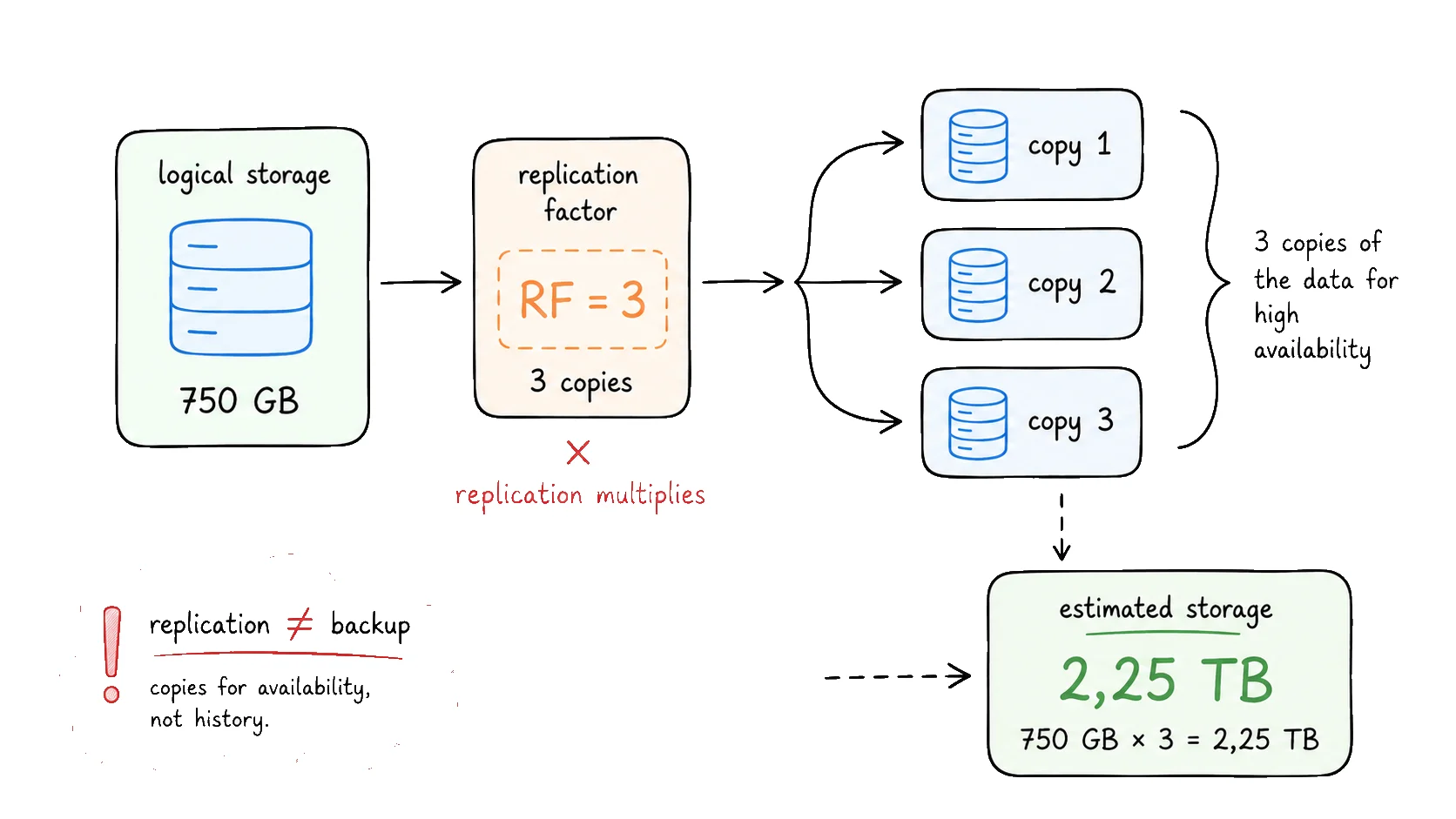
Replication means keeping more than one copy of the data to increase availability, durability, or fault tolerance.
Instead of depending on a single disk, node, or zone, the system keeps additional copies. That way, if part of the infrastructure fails, another copy is still available.
The important point for our estimate is simple: each copy takes space.
If the logical volume is 750 GB and the system keeps three copies of the data, the calculation becomes:
Logical storage
Replication
Estimated storage
750 GB
×
3 copies
=
2.25 TB
Logical storage
750 GB
×
Replication
The same information is still being generated by the system. What changed was the number of copies kept to protect and serve that data.
That is why replication enters the calculation as a multiplier.
Logical storage
Replication factor
Replicated storage
accumulated volume
×
number of copies
=
estimated volume
Logical storage
accumulated volume
×
In this example, 750 GB already looked large, but still manageable. With three copies, the number becomes 2.25 TB.
This is where many initial estimates start becoming more realistic.
Replication is not backup
Replication protects against machine, disk, node, or zone failure — there is always another copy ready. But it does not protect against human error, bugs, or accidental deletion: those can propagate to every copy. Backup is different: it exists for historical recovery, with its own frequency, retention, and cost.
For the storage calculation, what matters is that these are different things — replication multiplies the active data volume; backup is separate storage with its own calculation. Backup is intentionally not included in this estimate: frequency, retention, and policy vary too much by company, contract, and compliance context to fit into a quick calculation. We continue only with replication; the other factors appear in the final cautions.
Now we can put together the main variables in the estimate.
In our example, we started with:
5 writes/s;
50 KB per write;
approximately 25 GB/day;
30 days of retention;
replication factor 3.
Daily volume
Retention
Replication
Estimated storage
25 GB/day
×
30 days
×
3 copies
=
2.25 TB
This is the most important point of the calculation: a small rate per second can become a large volume when accumulated over time and multiplied by copies.
The mental formula looks like this:
writes/s × average size × retention time × replication factor = estimated storage
The calculation we made helps reveal the order of magnitude, but it still does not represent the full real production usage.
Some factors can increase, reduce, or distort this number:
Factor
Effect on storage
Why
Indexes
increases
They improve queries, but also take space.
Backups and snapshots
increases
They create additional copies, with their own retention policies.
WAL, journal, or transaction log
increases
Databases keep internal records for recovery and consistency.
Compression
reduces
It may reduce stored volume, depending on the type of data.
Traffic peaks
distorts
The daily average may hide periods of higher data generation.
Future growth
distorts
Today's calculation may not represent the volume six months from now.
That is why this estimate should be treated as a starting point.
It helps make better decisions, ask questions earlier, and avoid surprises. But before committing to a budget, provisioning infrastructure, or defining operational limits, the ideal path is to validate the calculation with real system metrics.
Storage usually does not become a problem because of a single write.
It becomes a problem through accumulation: small records, events, logs, and history generated every day, for weeks, months, or years.
The estimate does not need to be perfect to be useful. Starting with writes/s, average size, retention time, and replication factor already helps reveal the order of magnitude before growth becomes cost, a bottleneck, or an incident.
Later, with real metrics, the calculation can be refined.
The important thing is not to treat storage as infinite, and not to leave this conversation for the moment when the disk alert is already screaming in production.
Estimating storage is less about hitting the exact number and more about not being caught by surprise.
So here is the invitation: next time you launch a new service, sketch this napkin calculation before the first deploy. Five minutes now can save you from that bill shock later.
Average size
average size per write
=
Data generation
data generated per second
50 KB
=
Data generation
250 KB/s
Logical volume produced by the system before considering replication, indexes, backups, retention, or internal storage structures.
86,400 ≈ 100,000
A number that is easier to calculate mentally.
Scientific notation
100,000 = 10⁵
A more compact way to visualize it.
For our quick estimates: 1 day ≈ 100,000 seconds ≈ 10⁵ seconds
21.6 GB/day
Using the real 86,400 seconds in a day.
Difference
3.4 GB/day
Small in one day, but relevant when accumulated.
Approximation helps reveal the scale. A more precise calculation helps when the difference starts affecting cost, capacity limits, or operational decisions.
30 days
=
Logical storage
750 GB
Accumulated logical volume before considering replication, backups, indexes, snapshots, or storage overhead.
archival
Moved to cheaper storage for occasional lookup, audit, or history.
Expired data
safe deletion
Removed when there is no longer a retention need.
3 copies
=
Estimated storage
2.25 TB
Estimate considering three copies of the data. It still does not include backups, indexes, snapshots, WAL, journal, or other internal overheads.
Replication factor
number of copies
=
Replicated storage
estimated volume
Daily volume
25 GB/day
×
Retention
30 days
×
Replication
3 copies
=
Estimated storage
2.25 TB
The whole chain at once: from daily volume to estimated storage — still without considering backups, indexes, snapshots, WAL, or journal.
Question1/5
Why isn't total RPS a good basis for estimating storage?